ultralytics/docs/en/yolov5/tutorials/architecture_description.md

comments	description	keywords
true	Explore the architecture of YOLOv5, an object detection algorithm by Ultralytics. Understand the model structure, data augmentation methods, training strategies, and loss computation techniques.	Ultralytics, YOLOv5, Object Detection, Architecture, Model Structure, Data Augmentation, Training Strategies, Loss Computation

Ultralytics YOLOv5 Architecture

YOLOv5 (v6.0/6.1) is a powerful object detection algorithm developed by Ultralytics. This article dives deep into the YOLOv5 architecture, data augmentation strategies, training methodologies, and loss computation techniques. This comprehensive understanding will help improve your practical application of object detection in various fields, including surveillance, autonomous vehicles, and image recognition.

1. Model Structure

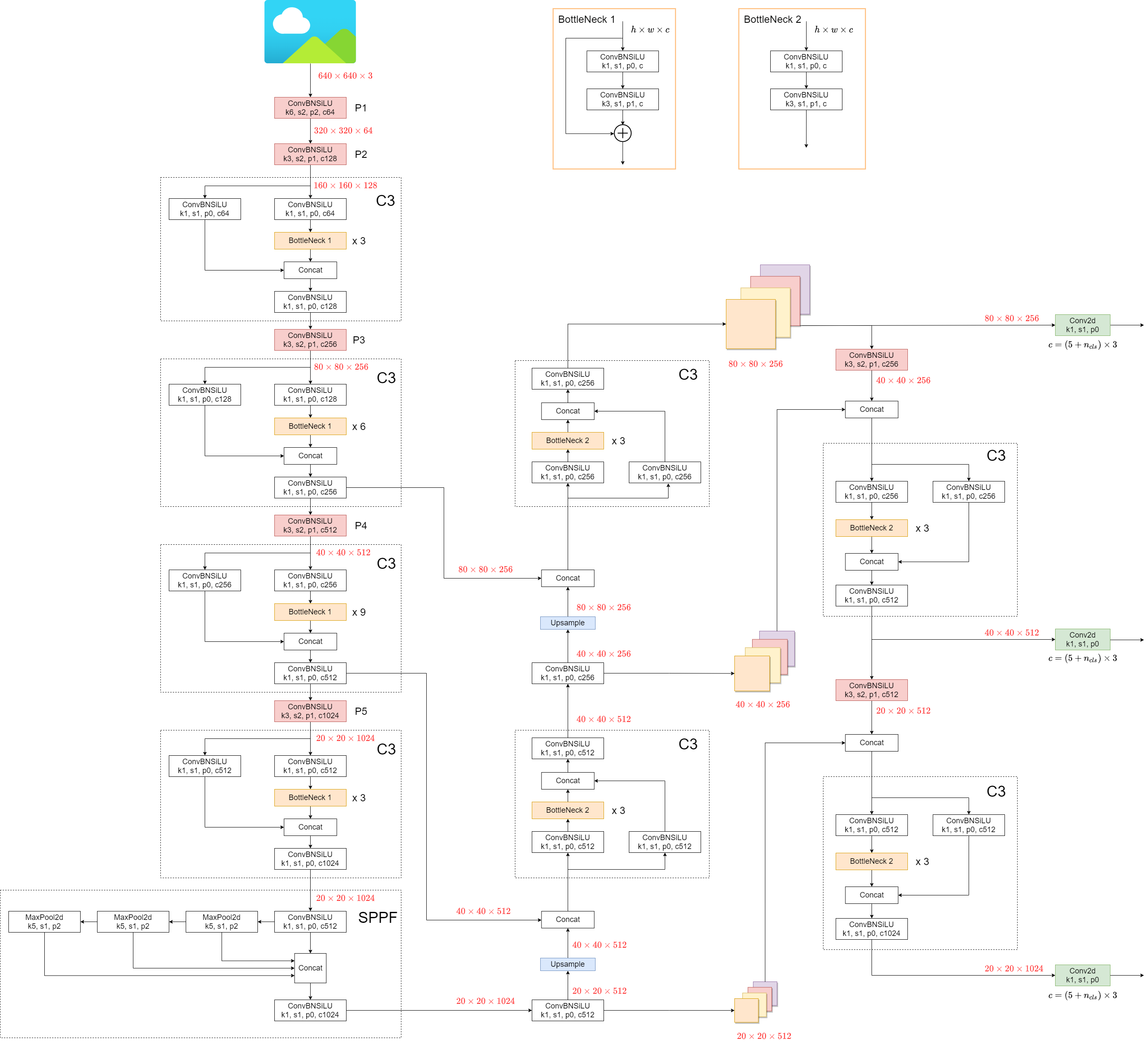
YOLOv5's architecture consists of three main parts:

• Backbone: This is the main body of the network. For YOLOv5, the backbone is designed using the New CSP-Darknet53 structure, a modification of the Darknet architecture used in previous versions.
• Neck: This part connects the backbone and the head. In YOLOv5, SPPF and New CSP-PAN structures are utilized.
• Head: This part is responsible for generating the final output. YOLOv5 uses the YOLOv3 Head for this purpose.

The structure of the model is depicted in the image below. The model structure details can be found in yolov5l.yaml.

YOLOv5 introduces some minor changes compared to its predecessors:

1. The Focus structure, found in earlier versions, is replaced with a 6x6 Conv2d structure. This change boosts efficiency #4825.
2. The SPP structure is replaced with SPPF. This alteration more than doubles the speed of processing.

To test the speed of SPP and SPPF, the following code can be used:

SPP vs SPPF speed profiling example (click to open)

import time

import torch
import torch.nn as nn


class SPP(nn.Module):
    def __init__(self):
        """Initializes an SPP module with three different sizes of max pooling layers."""
        super().__init__()
        self.maxpool1 = nn.MaxPool2d(5, 1, padding=2)
        self.maxpool2 = nn.MaxPool2d(9, 1, padding=4)
        self.maxpool3 = nn.MaxPool2d(13, 1, padding=6)

    def forward(self, x):
        """Applies three max pooling layers on input `x` and concatenates results along channel dimension."""
        o1 = self.maxpool1(x)
        o2 = self.maxpool2(x)
        o3 = self.maxpool3(x)
        return torch.cat([x, o1, o2, o3], dim=1)


class SPPF(nn.Module):
    def __init__(self):
        """Initializes an SPPF module with a specific configuration of MaxPool2d layer."""
        super().__init__()
        self.maxpool = nn.MaxPool2d(5, 1, padding=2)

    def forward(self, x):
        """Applies sequential max pooling and concatenates results with input tensor; expects input tensor x of any shape."""
        o1 = self.maxpool(x)
        o2 = self.maxpool(o1)
        o3 = self.maxpool(o2)
        return torch.cat([x, o1, o2, o3], dim=1)


def main():
    """Compares outputs and performance of SPP and SPPF on a random tensor (8, 32, 16, 16)."""
    input_tensor = torch.rand(8, 32, 16, 16)
    spp = SPP()
    sppf = SPPF()
    output1 = spp(input_tensor)
    output2 = sppf(input_tensor)

    print(torch.equal(output1, output2))

    t_start = time.time()
    for _ in range(100):
        spp(input_tensor)
    print(f"SPP time: {time.time() - t_start}")

    t_start = time.time()
    for _ in range(100):
        sppf(input_tensor)
    print(f"SPPF time: {time.time() - t_start}")


if __name__ == "__main__":
    main()

result:

True
SPP time: 0.5373051166534424
SPPF time: 0.20780706405639648

2. Data Augmentation Techniques

YOLOv5 employs various data augmentation techniques to improve the model's ability to generalize and reduce overfitting. These techniques include:

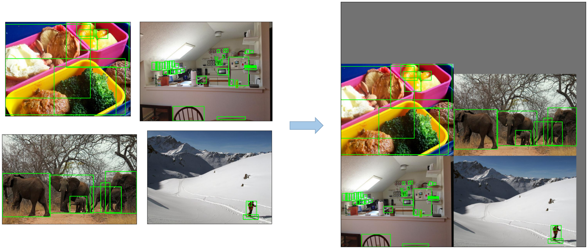
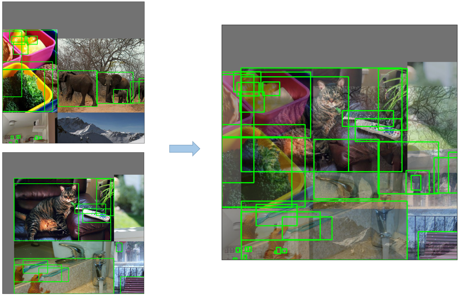
• Mosaic Augmentation: An image processing technique that combines four training images into one in ways that encourage object detection models to better handle various object scales and translations.

  

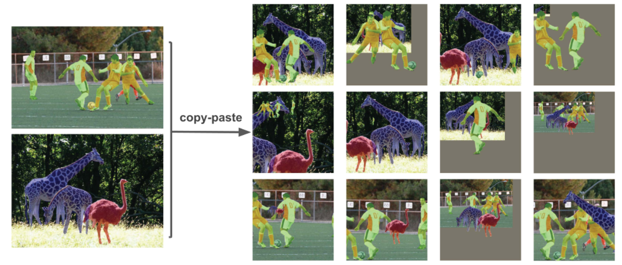
• Copy-Paste Augmentation: An innovative data augmentation method that copies random patches from an image and pastes them onto another randomly chosen image, effectively generating a new training sample.

  

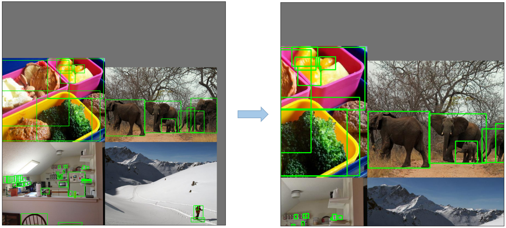
• Random Affine Transformations: This includes random rotation, scaling, translation, and shearing of the images.

  

• MixUp Augmentation: A method that creates composite images by taking a linear combination of two images and their associated labels.

  

• Albumentations: A powerful library for image augmenting that supports a wide variety of augmentation techniques.

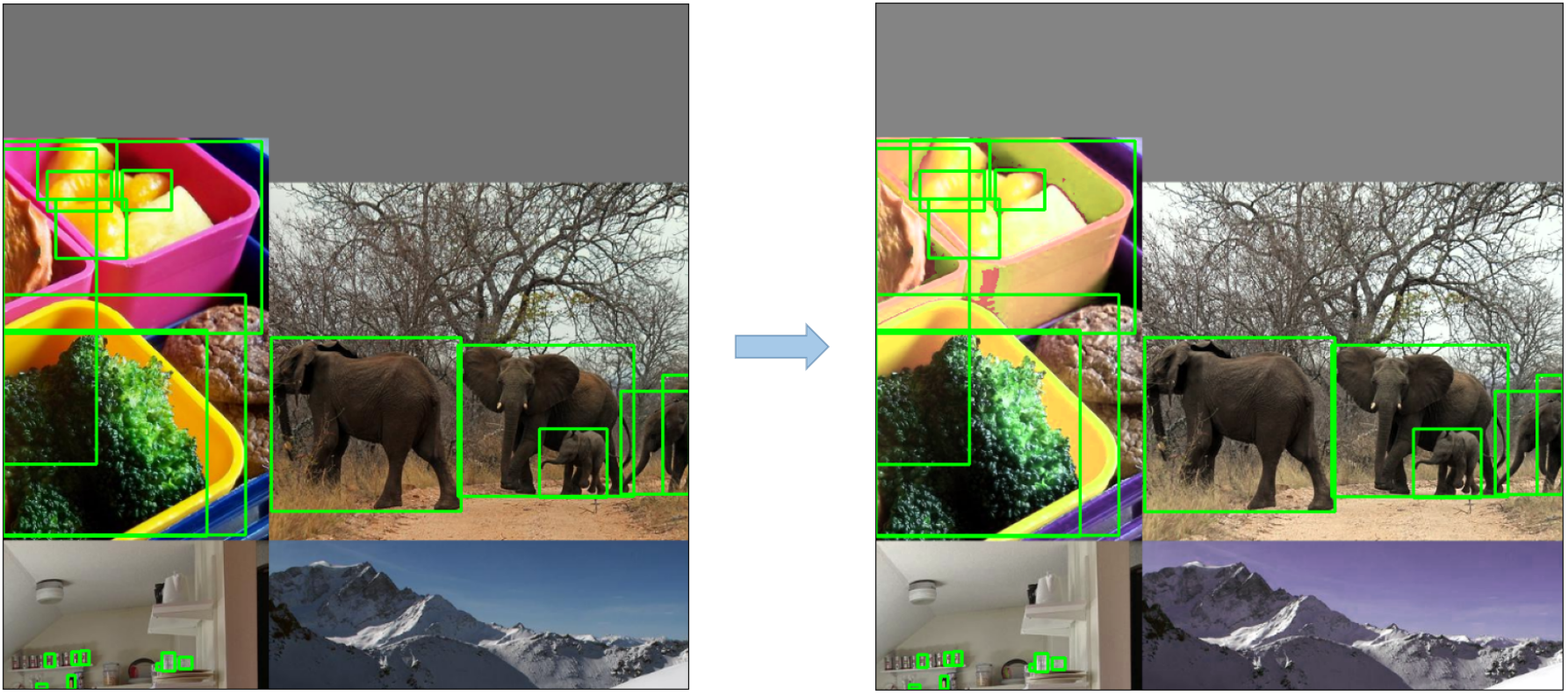
• HSV Augmentation: Random changes to the Hue, Saturation, and Value of the images.

  

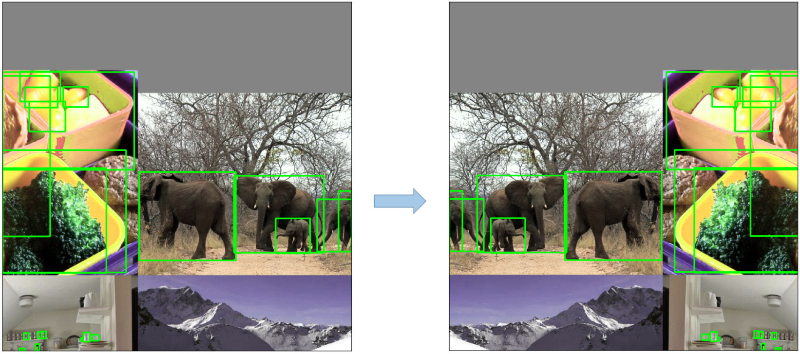
• Random Horizontal Flip: An augmentation method that randomly flips images horizontally.

  

3. Training Strategies

YOLOv5 applies several sophisticated training strategies to enhance the model's performance. They include:

• Multiscale Training: The input images are randomly rescaled within a range of 0.5 to 1.5 times their original size during the training process.
• AutoAnchor: This strategy optimizes the prior anchor boxes to match the statistical characteristics of the ground truth boxes in your custom data.
• Warmup and Cosine LR Scheduler: A method to adjust the learning rate to enhance model performance.
• Exponential Moving Average (EMA): A strategy that uses the average of parameters over past steps to stabilize the training process and reduce generalization error.
• Mixed Precision Training: A method to perform operations in half-precision format, reducing memory usage and enhancing computational speed.
• Hyperparameter Evolution: A strategy to automatically tune hyperparameters to achieve optimal performance.

4. Additional Features

4.1 Compute Losses

The loss in YOLOv5 is computed as a combination of three individual loss components:

• Classes Loss (BCE Loss): Binary Cross-Entropy loss, measures the error for the classification task.
• Objectness Loss (BCE Loss): Another Binary Cross-Entropy loss, calculates the error in detecting whether an object is present in a particular grid cell or not.
• Location Loss (CIoU Loss): Complete IoU loss, measures the error in localizing the object within the grid cell.

The overall loss function is depicted by:

4.2 Balance Losses

The objectness losses of the three prediction layers (P3, P4, P5) are weighted differently. The balance weights are [4.0, 1.0, 0.4] respectively. This approach ensures that the predictions at different scales contribute appropriately to the total loss.

4.3 Eliminate Grid Sensitivity

The YOLOv5 architecture makes some important changes to the box prediction strategy compared to earlier versions of YOLO. In YOLOv2 and YOLOv3, the box coordinates were directly predicted using the activation of the last layer.

However, in YOLOv5, the formula for predicting the box coordinates has been updated to reduce grid sensitivity and prevent the model from predicting unbounded box dimensions.

The revised formulas for calculating the predicted bounding box are as follows:

Compare the center point offset before and after scaling. The center point offset range is adjusted from (0, 1) to (-0.5, 1.5). Therefore, offset can easily get 0 or 1.

Compare the height and width scaling ratio(relative to anchor) before and after adjustment. The original yolo/darknet box equations have a serious flaw. Width and Height are completely unbounded as they are simply out=exp(in), which is dangerous, as it can lead to runaway gradients, instabilities, NaN losses and ultimately a complete loss of training. refer this issue

4.4 Build Targets

The build target process in YOLOv5 is critical for training efficiency and model accuracy. It involves assigning ground truth boxes to the appropriate grid cells in the output map and matching them with the appropriate anchor boxes.

This process follows these steps:

• Calculate the ratio of the ground truth box dimensions and the dimensions of each anchor template.

• If the calculated ratio is within the threshold, match the ground truth box with the corresponding anchor.

• Assign the matched anchor to the appropriate cells, keeping in mind that due to the revised center point offset, a ground truth box can be assigned to more than one anchor. Because the center point offset range is adjusted from (0, 1) to (-0.5, 1.5). GT Box can be assigned to more anchors.

This way, the build targets process ensures that each ground truth object is properly assigned and matched during the training process, allowing YOLOv5 to learn the task of object detection more effectively.

Conclusion

In conclusion, YOLOv5 represents a significant step forward in the development of real-time object detection models. By incorporating various new features, enhancements, and training strategies, it surpasses previous versions of the YOLO family in performance and efficiency.

The primary enhancements in YOLOv5 include the use of a dynamic architecture, an extensive range of data augmentation techniques, innovative training strategies, as well as important adjustments in computing losses and the process of building targets. All these innovations significantly improve the accuracy and efficiency of object detection while retaining a high degree of speed, which is the trademark of YOLO models.